
Special Report: Q-CTRL's Practical Quantum Advantage
3000x faster on the 1D Fermi-Hubbard simulation on IBM Heron. Is quantum advantage here? (and is superconducting back???)

This is a special-format post on Q-CTRL’s announcement, devoted to this single result rather than another modality piece because it’s an excellent conversation on framing quantum advantage. The analysis here draws on the technical paper and announcement materials alongside a pre-publication briefing with Q-CTRL Founder & CEO Michael Biercuk, VP of Quantum Computing Research Yuval Baum, and Senior Research Scientist Gavin Hartnett.
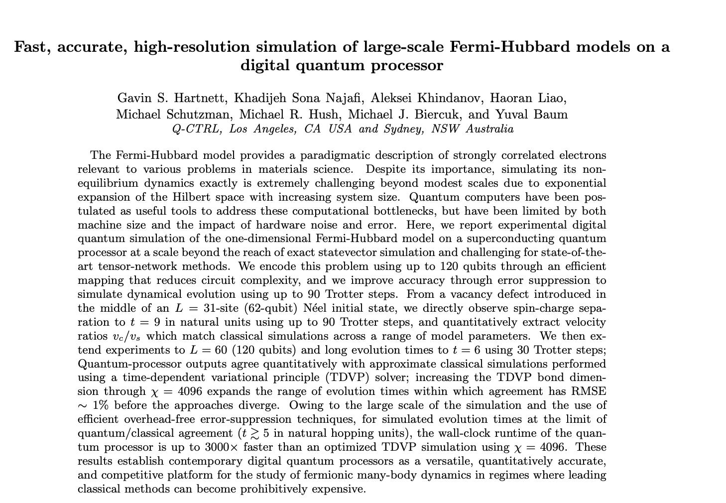
Today Q-CTRL is announcing what they’re calling the first Practical Quantum Advantage: a 1D Fermi-Hubbard simulation on IBM’s ibm_boston Heron processor that completes a meaningful materials-physics calculation in roughly two minutes wall-clock against an industry-standard tensor-network calculation that took over 100 hours on a 32-core CPU node (Hartnett et al., 2026).
Scientists and engineers dedicate thousands of hours to performing materials simulations in their efforts to unlock the future of energy, from photovoltaics to fusion. These results mark the beginning of an era of positive ROI from today’s widely available quantum computers on problems that early adopters truly care about. That’s the nature of Practical Quantum Advantage.
- Michael J. Biercuk, CEO and Founder of Q-CTRL
The headline number being put out is up to 3000x faster, calculated at the regime where the two methods last agreed within tolerance.
This paper lands on the timeline of Jay Gambetta’s previously stated commitment that IBM would demonstrate quantum advantage this year, and Q-CTRL has been careful about defining their term. Those choices shape what “Practical Quantum Advantage” means for the industry.
“Is quantum here?” That’s the wrong question.
A better question is:
Given the tools available to me today, is the quantum route faster or better for a problem I actually care about?
What Q-CTRL actually did
What did Q-CTRL actually solve? The Fermi-Hubbard model is the simplest mathematical description of electrons that interact strongly enough that you can’t pretend they ignore each other. This is where conventional materials simulation breaks down. Density functional theory (DFT) works extremely well across large parts of semiconductor physics, conventional materials modeling, and molecular chemistry, but it is not reliable as a standalone tool for many strongly correlated systems. It does not get you through high-temperature superconductors, transition-metal oxides, or the materials underlying most of the open problems in energy storage, catalysis, and quantum magnetism. Those are the systems where electron-electron repulsion is comparable to or larger than the kinetic energy, and where the standard approximations stop working.
That is not a niche set of problems. In the U.S. national-lab ecosystem, chemistry and materials simulation has been estimated to consume roughly a third of supercomputer time, and the open problems at the frontier of that workload — better cathode chemistries for batteries, room-temperature superconductor candidates, more selective catalysts, the magnetic materials underlying storage and sensing — are where DFT stops working. A faster, more accurate solver for the strongly correlated regime is economically consequential to materials problems sitting in industrial R&D right now.
Solving Fermi-Hubbard at scale is the canonical test of whether a computational tool can handle that regime. The 1D version is exactly solvable in equilibrium (via Bethe ansatz) and well-characterized dynamically by tensor network methods, which is why it’s the validation target. You can check the answer. The 2D version has resisted exact classical treatment for nearly four decades.
Five Fermi-Hubbard demonstrations have shipped in roughly six months:
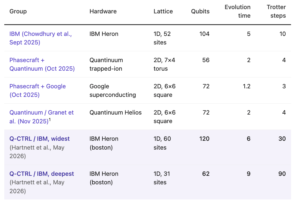
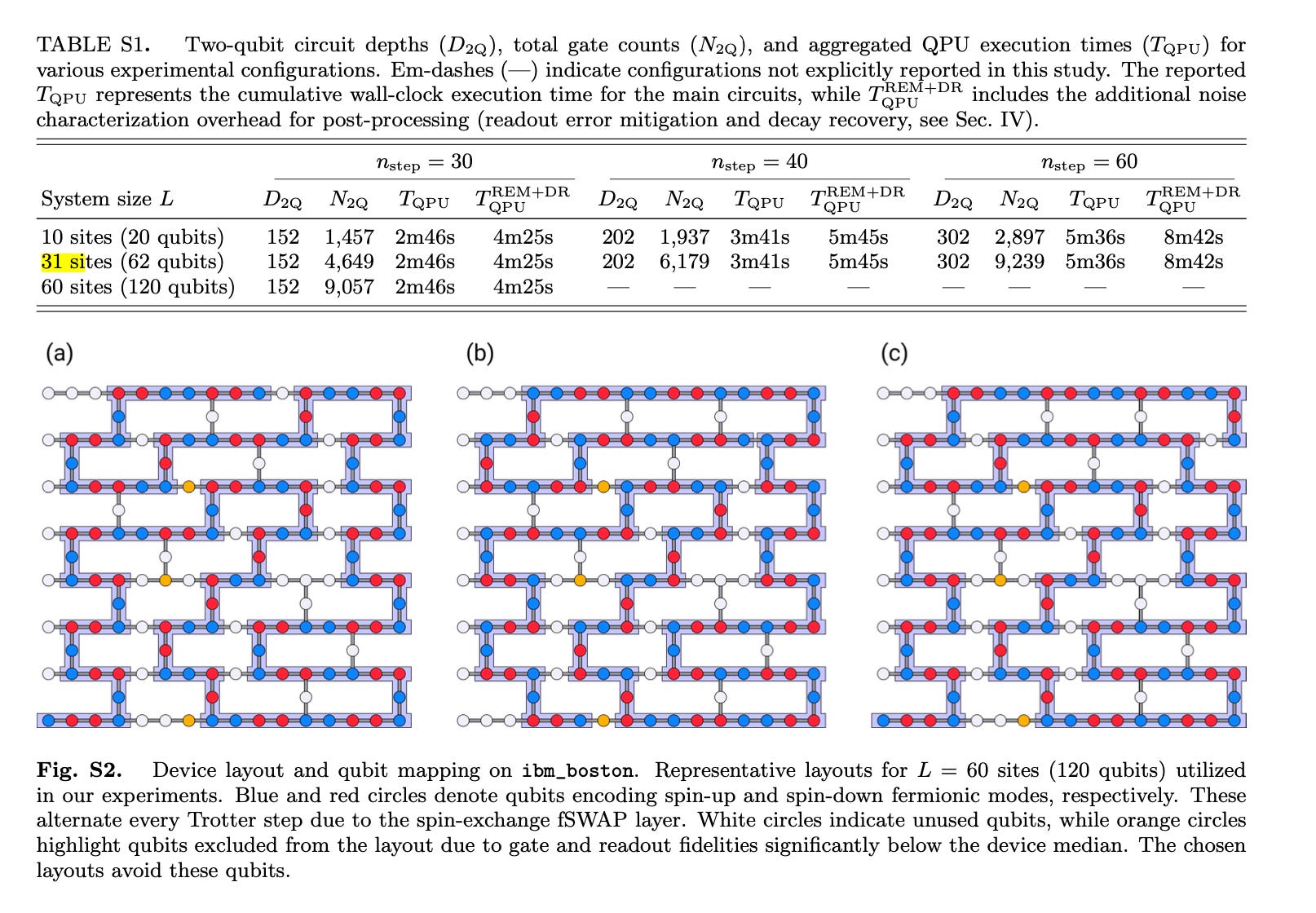
The team mapped the fermionic chain to qubits using a Jordan-Wigner transformation with a “pair-interleaved” ordering and an fSWAP network, and ran two flavors of experiment on ibm_boston (a 156-qubit Heron device (which has shorter T1 coherence times than some of its predecessors): a widest configuration of L = 60 sites (120 qubits) evolved to t = 6 in natural hopping units using 30 Trotter steps, and a deepest configuration of L = 31 sites (62 qubits) evolved to t = 9 using 90 Trotter steps. All experiments use 20,000 shots per circuit.
The widest circuits use 9,057 two-qubit gates organized into 152 layers. The deepest circuits push to over 13,800 two-qubit gates at a depth of 452 layers. For context, this is well past the 100-qubit × 100-layer “quantum utility” conceptual milestone IBM had previously held up as a marker for advantage demonstrations — a comparison Yuval Baum drew directly when walking me through the result.
Q-CTRL has the largest 1D system, the longest evolution time, and the most Trotter steps. Phasecraft has 2D demonstrations on both Google and Quantinuum hardware. Quantinuum’s own native paper uses trapped ions but measuring a different observable — superconducting pairing correlations across three regimes. IBM’s prior 52-site work was the immediate predecessor on this work.
Crucially: this was run on the public IBM API, with no special calibration — the same access path any IBM Quantum user has. Yuval Baum was emphatic about this in our briefing: “we ran it on the public API, exactly like any other user, we didn’t get any special calibration or attention or help from IBM.” Many prior quantum-advantage demonstrations involved bespoke calibration runs, dedicated device access, or otherwise non-reproducible experimental conditions.
The widest experiments report agreement with classical TDVP simulations using ITensorMPS.jl at χ = 4096 within ~1% RMSE (root-mean-square error) across all 120 spin-orbital occupations up to t ≈ 5.2. Beyond that point, the methods diverge; Q-CTRL describes correctness as indeterminate because there is no exact ground truth at that scale. Even at the longest evolution times tested, the residual quantum error stays around 4%. The community's accepted accuracy band for these dynamic simulations is generally 5–10%.
Q-CTRL is precise about what they mean by Practical Quantum Advantage
addresses a problem of known scientific or commercial value;
runs on a publicly accessible quantum computer;
uses no privileged hardware access;
is compared against the classical tool researchers actually use;
includes end-to-end wall-clock runtime, not just hardware execution time;
and produces results within the accuracy expectations of the application.
They explicitly do not claim absolute advantage over any conceivable classical algorithm.
They name the regime where both methods become unreliable.
They validate against analytic theory (Bethe ansatz) before pushing into the regime where the analytic doesn’t apply.
They consulted directly with the ITensor development team at the Flatiron Institute, the people who actually wrote the classical baseline they’re benchmarking against.
So a one-liner of the result is: “the largest 1D Fermi-Hubbard simulation, run on a publicly accessible quantum computer with no privileged access, faster end-to-end than the most-used classical tool in the materials community, validated by that tool’s own developers, with accuracy that exceeds the community’s normal tolerance.”
What the 3,000× number actually represents
The classical baseline is ITensor on a single 32-vCPU node (AWS c7i.8xlarge, 64 GB RAM). The ITensor team confirms there’s no GPU-accelerated path readily available for ITensorMPS.jl that incorporates the particle and spin conservation symmetries this problem requires, and parallelization gains plateau well below 32 cores. The team also empirically validates that doubling to 64 cores yields negligible improvement. Q-CTRL did test available GPU-based tensor-network packages directly. Baum confirmed in our briefing that they ran them and found them slower than the mature CPU implementation, because the GPU options are less developed for symmetry-adapted tensor networks. The paper itself acknowledges that future GPU acceleration, algorithmic improvements, or narrow-purpose tooling could close part of the gap, while noting that no such acceleration is readily available to the community today.
The wall-clock comparison is calculated at a specific point in evolution time: t ≈ 5.2, where TDVP at χ = 4096 last agrees with the quantum data within ~2% RMSE. At that point, for one specific simulation:
Quantum: ~2 minutes, total end-to-end (compilation, communication latency, hardware execution over 20,000 shots per circuit, post-processing).
TDVP χ = 4096: ~100 hours on the 32-core CPU node.
Three things to note:
First, the comparison is calibrated against the agreement boundary. At t = 6 (the maximum evolution time tested), quantum is still ~2.5 minutes and classical exceeds 160 hours. At t = 4 (well before divergence), classical finishes in roughly 20 minutes against quantum’s ~1 minute, and the ratio collapses by orders of magnitude. The 3,000× is the most favorable point on a smoothly varying curve, taken where validation is still tight. Q-CTRL is clear they chose this point deliberately because it’s the last evolution time where they can confidently say the quantum result is correct.
Second, the comparison is per simulation. Materials scientists doing real work multiple values, multiple initial conditions, multiple lattice sizes. If you’re scanning ten values, classical takes 1,000 hours and quantum takes 25 minutes, with the same 3,000× ratio.
Third, quantum runtime grows linearly in number of Trotter steps. TDVP runtime scales as O(L · χ³) per step, with χ growing exponentially in entanglement entropy, which grows linearly in time before saturation. The classical curve bends sharply upward at long times. Quantum should grow more slowly than classical for this problem as evolution time increases.
The error-suppression stack
Q-CTRL is not selling Fermi-Hubbard simulation. They’re selling Fire Opal, a runtime infrastructure layer that wraps the hardware and improves circuit fidelity through a stack of techniques. The Fermi-Hubbard result is the demonstration of what simulations can be pushed when that stack is executed at scale.
I asked the Q-CTRL team what they think were the keys to what they did differently.
Three things:
They don’t build algorithms; they build the tools to run algorithms well. Q-CTRL used application-aware compilation. Instead of handing a generic fermionic simulation circuit to a generic transpiler, they optimized the mapping and circuit structure for this Hamiltonian, this device topology, and this observable set. In the manuscript, Q-CTRL reports more than 60% fewer two-qubit gates and more than 80% lower two-qubit-layer depth compared with a Qiskit Nature plus Qiskit transpiler baseline.
They suppress errors at runtime rather than mitigating them via measurement-overhead-heavy post-processing. On a 120-qubit circuit, bad qubits matter. Q-CTRL’s stack — layout selection, dynamical decoupling, Pauli twirling, readout mitigation, amplitude-decay recovery — keeps measurement overhead constant. For a 120-qubit circuit on ibm_boston, only 21 of roughly 109,000 possible layouts avoid the device’s three persistently high-noise qubits. Picking that layout is a massive advantage and overall drives costs down and makes the quantum computer more useful.
They picked a problem people actually care about and benchmarked it against the tool people actually use. In our briefing, Baum was explicit about how Q-CTRL views the prior 2025/2026 Fermi-Hubbard demonstrations: as benchmarks of device capability rather than solutions of the simulation problem. At the short evolution times those works probe, the system hasn’t yet developed enough entanglement to challenge classical methods, and the comparison becomes about circuit execution rather than physical insight. Whether the Phasecraft, Google Quantum AI, and Quantinuum teams accept that characterization is a separate question.
The advantage Q-CTRL did not claim: economic
Practical advantage means the quantum solution is faster end-to-end than the alternative researchers actually use. Economic advantage means a customer would pay for the quantum solution at a price that makes commercial sense for both sides — i.e., that the cost-per-useful-result on quantum is competitive with or cheaper than the classical cost-per-useful-result, accounting for everything: compute time, software licensing, integration cost, switching cost, and the value of the answer to the buyer.
Practical advantage is necessary for economic advantage as of this time, as quantum computers are pretty expensive; but it’s not sufficient. Economic advantage depends on the cost-per-useful-result: quantum access, software licensing, integration, switching cost, trust, and the value of the answer to the buyer. But, as we have seen in AI, some customers will tolerate high compute costs when faster or better results change time-to-market, but will this apply to materials workflows? It may not matter in the end because of the potential unknown value of what these results can lead to.
What I’d watch next
The commercial test: whether materials scientists who currently use ITensor every day will actually adopt a Fire Opal Qiskit Function for production work. Scientific advantage on a benchmark is one thing; the migration of an installed base is another. Q-CTRL’s own announcement materials note that ITensor has been used in “over 1,250 technical publications in the field of quantum materials since its release in 2015, including around 200 last year”. Usage is accelerating, not declining, so this is a useful library and application.
Expect scrutiny. The skeptic community will press hard on the 1D-vs-2D point, on the choice of classical baseline, and on whether 1D Fermi-Hubbard advantage extrapolates to anything that materials engineers actually care about, and which configurations of hardware, compilation, and error suppression will sustain advantage as problems get harder, and whether the end users will pick it up.
Q-CTRL’s methodology is designed to build that trust gradually: validate where you can, push where you must, and be explicit about where correctness becomes indeterminate. If the quantum computer and the classical method disagree, and no exact answer exists, who do you believe?